Background Governance

Compaction and Flush Strategies

Before discussing compaction, it is essential to understand three key concepts:

Read Amplification: The actual amount of data read exceeds the logical data size. For example, an LSM-Tree query may need to scan multiple SSTables to retrieve a single key.
Write Amplification: The actual amount of data written to disk exceeds the logical data size. For instance, writing a single key in an LSM-Tree might trigger a compaction operation, causing significantly more data to be rewritten.
Space Amplification: The actual disk space occupied is larger than the logical data size. This often occurs when old, invalid versions of data remain stored in SSTables.

LSM-Trees achieve high write throughput through sequential writes and background compaction. The compaction strategy determines the core trade-off between write performance, read performance, and resource consumption. Traditional LSM-Trees primarily use two compaction strategies: Size-Tiered Compaction and Level Compaction.

Tiering: Accumulates files first, then merges them in batches once a threshold is reached (write-optimized). Think of this as tossing files into a drawer and archiving them only when full.
Leveling: Keeps every level sorted and organized, preventing disorder (read-optimized). Think of this as immediately placing every file onto a clearly categorized shelf.

Tiered Compaction (RocksDB)

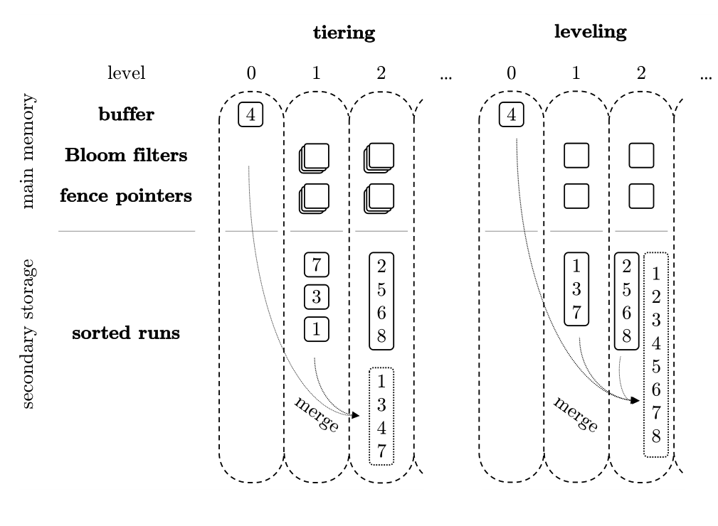
In this strategy, SSTables within the same level are allowed to overlap. Similar-sized SSTables are batched together into larger SSTables without strictly enforcing non-overlapping ranges per level.

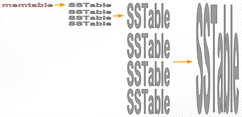
Advantages: Low write amplification (merges are more opportunistic; data is not repeatedly rewritten just to eliminate overlaps).
Disadvantages: High read amplification (queries may need to scan multiple Runs).

The Size-Tiered Compaction Strategy (STCS) merges SSTables of similar sizes into a new file. As memtables flush to disk as SSTables, they start as small files. As the number of small files grows and reaches a threshold, STCS compacts them into medium-sized files. Similarly, when the number of medium files reaches a threshold, they are compacted into large files. This recursive process continuously generates increasingly larger files.

Core Principles:

Multiple SSTables with overlapping key ranges are allowed within the same level.
Files accumulate first; a unified merge occurs only when a count threshold is reached.

Example: Assume each SSTable holds 4 keys.

First Flush: SST-A: [1 – 4]
Second Flush: SST-B: [5 – 8]
Third Flush (updates + new data): Writes keys 3, 6, 9, 10. Generates SST-C: [3 – 10].

Level 0 Structure: [1–4], [5–8], [3–10]

C overlaps with A on keys 3–4.
C overlaps with B on keys 5–8.

Querying key=6 requires scanning multiple files, illustrating read amplification. In Tiered compaction, a merge is triggered when the file count in a level hits a threshold, outputting a single large file (e.g., [1 – 10]). Thus, the advantage is fast writes with low write amplification, but the disadvantage is that queries must scan multiple files, resulting in read amplification.

Leveling Compaction (Cassandra)

SSTables within each level strive to be non-overlapping (disjoint key ranges). If an overlap occurs, the upper-level SSTable and all overlapping lower-level SSTables are merged and rewritten.

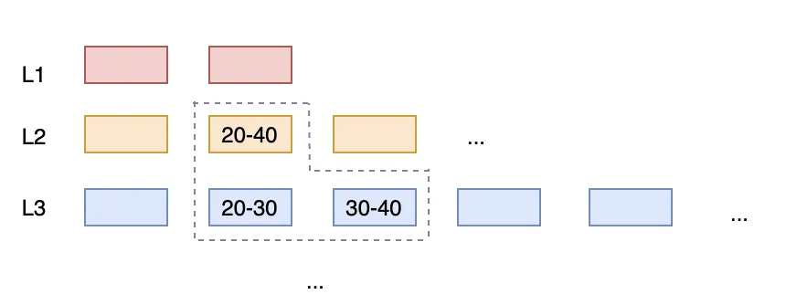
Advantages: Low read amplification (querying a key or range typically requires scanning very few files).
Disadvantages: High write amplification (frequent rewriting of large data volumes).

In Leveled compaction, each level consists of ordered Runs of SSTables, maintaining sorted relationships between them. When a level's data size reaches its limit, it merges with the Run in the next level. This approach reduces the number of Runs per level, minimizing read and space amplification. The use of small SSTables allows for granular task splitting and control, where controlling task size effectively controls temporary space usage.

Core Principles:

SSTable key ranges within each level must be non-overlapping.
The entire system forms a continuous, ordered space.

Example: Using the same scenario, upon detecting overlaps ([1–4], [5–8], [3–10]), an immediate merge occurs to produce [1–10]. This is then split into [1–5] and [6–10] to ensure non-overlapping intervals within the level. Thus, the advantage is fast queries (scanning at most one file), but the disadvantage is high write amplification, continuous background compaction, and heavy I/O pressure.

Dimension	Tiered	Leveling
Overlap within Level	Allowed	Not Allowed
Write Cost	Very Low	Medium-High
Query Cost	High	Very Low
Write Amplification	Low	High
I/O Pressure	Light	Heavy
Latency Stability	Poor	Good
Primary Goal	Throughput	Response Time

MARS3 Implementation

MARS3 adopts a Tiered Compaction strategy. In typical time-series workloads (VIN + TS), continuous writes cause new Runs to widely overlap with multiple Runs in lower levels regarding key space. Maintaining non-overlapping levels with Leveled Compaction becomes difficult, frequently triggering large-scale rewrites. This results in significant write amplification, which is further exacerbated in MPP multi-instance scenarios.

Scenario: Assume three devices (VIN=A, B, C) continuously report latest values. The system already has a Level 1 (L1) layer where each file covers a specific time range for a VIN:

Existing L1:
- A History: A:[0 ~ 999], A:[1000 ~ 1999]
- B History: B:[0 ~ 999], B:[1000 ~ 1999]
- C History: C:[0 ~ 999], C:[1000 ~ 1999]

New Data Arrives:

A reports: TS = 1500 ~ 1700
B reports: TS = 1600 ~ 1800
C reports: TS = 1400 ~ 1650

These new writes form a new Run (e.g., in L0 or an upper level), called NewRun. NewRun contains the latest time slices for A, B, and C, covering approximately:

A:[1500 ~ 1700]
B:[1600 ~ 1800]
C:[1400 ~ 1650]

Overlap Analysis:

A's new data overlaps with A:[1000 ~ 1999].
B's new data overlaps with B:[1000 ~ 1999].
C's new data overlaps with C:[1000 ~ 1999].

Consequently, a single NewRun overlaps with multiple L1 files (one per VIN). If there are 10,000 VINs writing simultaneously, one NewRun could overlap with hundreds or thousands of L1 files. Leveled Compaction requires L1 files to be non-overlapping. Therefore, merging NewRun into L1 would require reading NewRun plus all overlapping L1 files, re-sorting them, and writing new L1 files to maintain the non-overlapping property. Even if the new write is small (e.g., 1 GB), if it touches many historical segments, it drags in massive amounts of historical data (e.g., 10 GB, 50 GB, or 100 GB) for rewriting, causing severe write amplification.

In contrast, Size-Tiered Compaction does not enforce non-overlapping lower levels. It primarily merges Runs of similar sizes. It does not drag in大量 lower-level files solely to eliminate overlaps. Thus, in this scenario, write amplification is significantly reduced.

Furthermore, MARS3 Runs are columnar structures requiring sufficient physical continuity to ensure scan throughput and compression efficiency. This conflicts with the small SSTable granularity often used in Leveled Compaction. Size-Tiered Compaction better fits this workload: it merges same-sized Runs, significantly reducing write amplification. Additionally, under time-progressive data streams, it naturally forms time-clustered Run organizations, making time-based filtering and skip-scans more effective.

To control read amplification, MARS3 limits the read amplification factor per level. Once this factor is exceeded, compaction to the lower level is triggered.

The parameter level_size_amplifier specifies the amplification factor for Level sizes. The threshold for triggering a merge at a specific level is calculated as: rowstore_size * (level_size_amplifier ^ (level - 1)).

A larger value results in slower reads but faster writes.
The value should be determined based on specific workload characteristics (write-heavy vs. read-heavy, compression ratios, etc.).
Caution: Ensure the number of Runs per level does not become excessive, as this degrades query performance and may even block new data inserts.

Essentially, level_size_amplifier controls how much larger each level can be compared to the previous one. Upper levels act as buffers, while lower levels serve as long-term storage.

Larger Amplifier: Levels can accumulate data longer, leading to more Runs. This increases the number of objects checked during queries (higher read amplification) but reduces compaction frequency (faster writes).
Smaller Amplifier: Triggers sinking and organization earlier, resulting in fewer, cleaner Runs. This improves read speed but increases compaction frequency.

Together, rowstore_size and level_size_amplifier create a controllable sinking rhythm. This constrains Run accumulation within the Tiered model, limiting read amplification while preserving write throughput advantages. See Observability for more details.

Compaction Scheduler

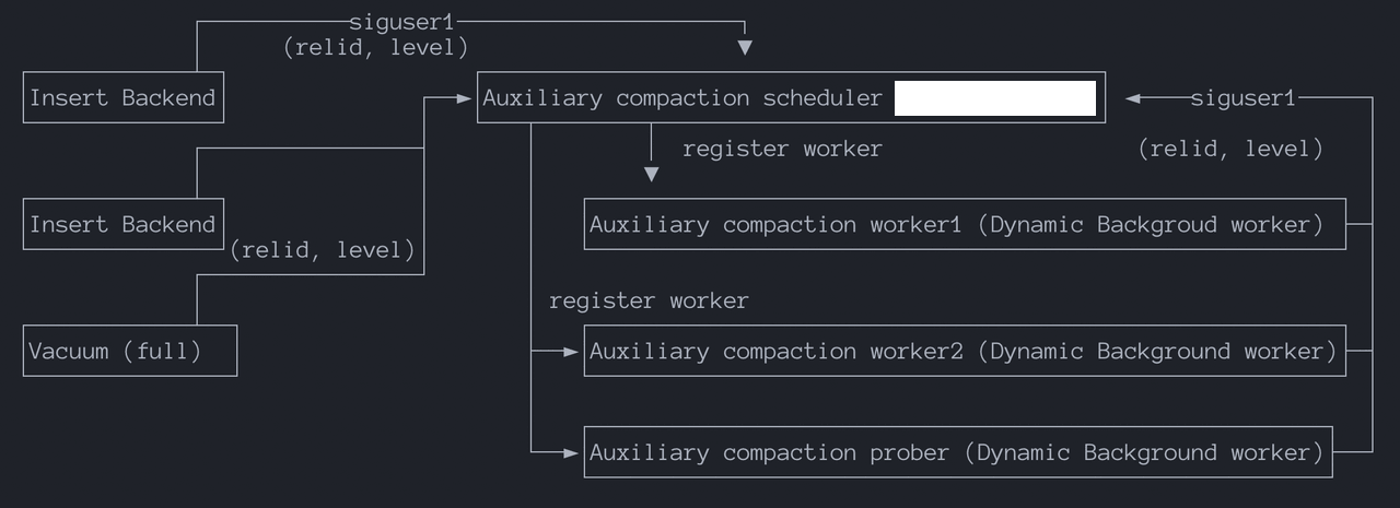
Compaction Scheduler: A persistent auxiliary process started upon database launch. When a rowstore reaches rowstore_size, the system switches to a new rowstore. A signal is sent to the scheduler process via shared memory, containing the compaction request details (relation ID and level). The scheduler is responsible for registering new workers to perform compaction.
- Responsibilities:
  - Start and stop compaction workers.
  - Manage and reuse compaction workers.
  - Determine compaction task priorities.
  - Correctly respond to database shutdown requests.
Compaction Worker: Executes specific compaction requests. If a level's read amplification exceeds the limit, the worker notifies the scheduler of a new compaction request. Due to current process model constraints, the maximum number of Compaction Workers is hardcoded to 16.
Compaction Prober: Actively probes for compaction tasks, such as:
- Scheduled compaction tasks.
- Interrupted compaction tasks.
- Workflow:
  1. Insert Backend continuously writes to RowStore.
  2. When a RowStore reaches the threshold, it switches to a new RowStore.
  3. Sends SIGUSR1 to the scheduler and writes compaction request info (relid, level) to shared memory.
  4. The scheduler wakes up, reads the request from shared memory:
    - Queues, deduplicates, and prioritizes requests.
    - Selects a new worker or reuses an idle one.
  5. The worker begins executing compaction.

Compaction Priority

When multiple tables require compaction but only 16 workers are available, a priority mechanism ensures the "most needy" tables are compacted promptly. Priority considerations include:

Level Hierarchy: Lower levels have higher priority.
Eager vs. Lazy: Manual vs. automatic triggers.
Compaction Type.

Autoprobe

Autoprobe periodically scans all MARS3 tables, calculating a score based on transaction age divided by size (age / size). It selects the top N levels with the highest scores to trigger flush/compaction tasks, effectively compressing historical levels. The function matrixts_internal.mars3_autoprobe_candidates() displays candidate levels and their scores:

adw=# SELECT * FROM matrixts_internal.mars3_autoprobe_candidates();
 segid | datname |   relname   | level | nruns |    age     |   bytes   |         score
-------+---------+-------------+-------+-------+------------+-----------+-----------------------
     0 | adw     | t_w0_nosort |     1 |    13 |     616005 |  49888440 |  0.012347650076851471
     0 | adw     | t_w0_nosort |     0 |     1 | 2147483647 |  25034752 |     85.78010467209741
     0 | adw     | t_w3b_3key  |     0 |     1 | 2147483647 |  25034752 |     85.78010467209741
     0 | adw     | t_w1_1key   |     1 |     7 |     329693 |  23821378 |  0.013840215288972788
...

Since Autoprobe always selects the highest-scoring levels, a blacklist mechanism prevents failure loops. If a compaction fails 3 times for the same level, it is added to the blacklist and no longer retried.

mars3_autoprobe_blacklist(): View the blacklist.
mars3_autoprobe_blacklist_remove(regclass, level): Remove a specific level from the blacklist for the current database.
mars3_autoprobe_blacklist_clear(): Clear the entire blacklist.

GUC Parameters:

mars3.autoprobe_period: Controls the probe interval in seconds. Value > 0 enables it; 0 disables it (default). Start with 10 minutes and adjust based on workload.
mars3.autoprobe_workers: Controls how many levels are selected per probe (default: 2). Note: These occupy standard compaction worker slots; no new workers are spawned.
mars3.autoprobe_retry: Controls retry attempts. A value of 2 means 3 total attempts.
mars3.autoprobe_blacklist_size: Controls the maximum size of the blacklist.

Impact of Disabling Autoprobe: Tables with no new writes will not undergo compaction. Tables with active writes will continue to merge normally.

Observability

Verify worker status:

ps aux | grep postgres | grep 'compact worker'

Check if all workers are running. Look for processes that have been running for a long time without exiting, which may indicate abnormal system behavior.

Database logs also contain compaction activity information. Create a table t1 and continuously insert data:

postgres=# CREATE TABLE t1(id int, info text)
USING mars3 WITH(mars3options='prefer_load_mode=single,rowstore_size=64');
NOTICE:  Table doesn't have 'DISTRIBUTED BY' clause -- Using column named 'id' as the Greenplum Database data distribution key for this table.
HINT:  The 'DISTRIBUTED BY' clause determines the distribution of data. Make sure column(s) chosen are the optimal data distribution key to minimize skew.
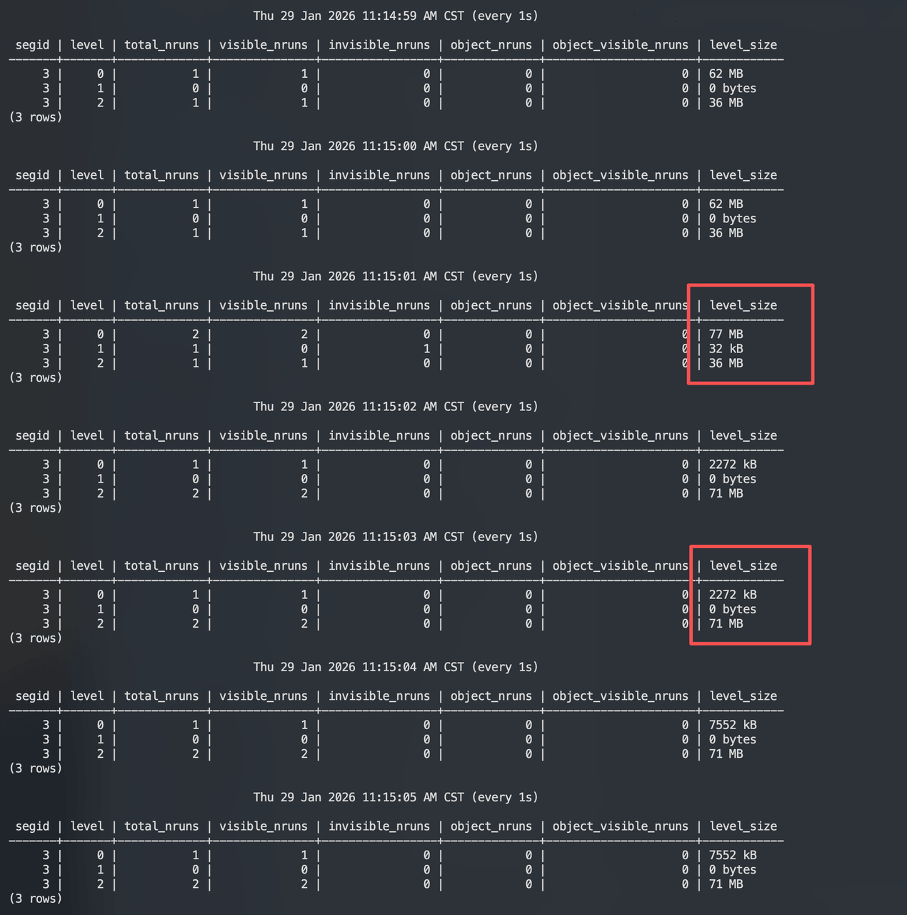
CREATE TABLE

Open a new window and continuously monitor level states using matrixts_internal.mars3_level_stats:

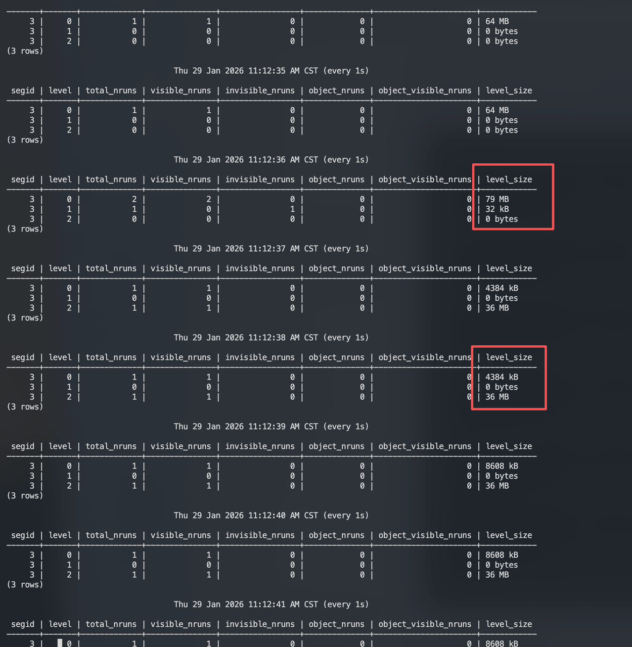
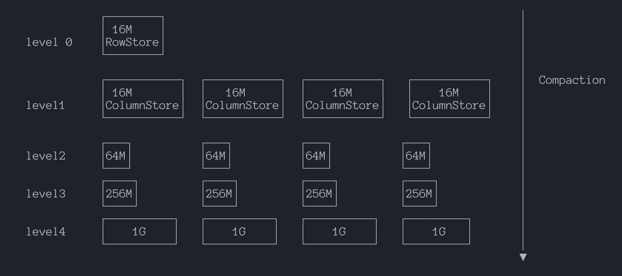
Observation: After L0 fills to 64 MB (rowstore_size), L1 briefly shows 32 KB, and data is written directly to L2. Subsequent writes also go directly to L2. Why not write to L1 first?

MARS3 includes an "Adjust Level" logic (GetDesiredLevel):

Calculates the target level (desired_level) for a Run based on its TotalSize.
If the current level (cur_level) differs, it locks the Run and moves it to the target level.

Calculation Flow:

run_size ≈ rowstore_size = 64 MB.
total_amp = run_size / rowstore_size = 64 MB / 64 MB = 1.0.
desired_level = log(1.0) / log(8) = 0.

The theoretical relative level is 0.

if (desired_level < 0) {
    ret = desired_level < -0.5 ? 1 : 2;
} else {
    ret = Min(2 + round(desired_level), MAXLEVELS - 1);
}

Since desired_level = 0, the else branch executes:

round(0) = 0.
ret = 2 + 0 = 2 (subject to Min upper bound protection).

Result: GetDesiredLevel() returns 2. According to the new rules, a 64 MB Run belongs in L2.

Design Principles

In MARS3's Tiered model, stable geometric growth is achieved not by strictly enforcing total size per level instantly, but by allowing compaction to gradually align Run target sizes with the amplifier factor. The core thresholds for triggering compaction are:

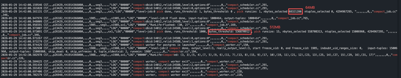
Old Version (< REL_V1): threshold(level) = rowstore_size × amp^level
New Version (>= REL_V1): threshold(level) = rowstore_size × amp^(level - 1)

Here, bytes_threshold estimates the input set size for a compaction/pick operation. Compaction picks N Runs whose total_size approximates bytes_threshold. Calculated Thresholds (assuming rowstore_size=64MB, amp=8):

Level 1: 64 MB
Level 2: 512 MB
Level 3: 4 GB
Level 4: 32 GB
...

A Min(MAX_RUN_SIZE, ...) constraint is applied. If the calculated size exceeds MAX_RUN_SIZE, the limit is capped to prevent excessively large jobs or output Runs.

Design Motivations

Motivation A: Stabilize the Geometric Growth Model.
- rowstore_size represents rowstore granularity.
- L1+ stores compressed columnar data, where byte sizes vary significantly.
- Without shifting the baseline, applying the same formula rigidly could cause distortions: L1 shrinks due to compression → triggers erratic compaction rhythms → leads to uncontrolled read amplification or accumulation.
- The new version uses level-1 in the formula and adds +2 in Run classification to align the model baseline to more stable layers. Engineering principle: Do not use the most volatile layer as the ruler.
Motivation B: Exponential Task Scaling with Upper Bounds.
- Exponential Growth: Deeper levels should handle larger data volumes per merge to avoid frequent disturbances to deep data (which causes write amplification and I/O jitter).
- MAX_RUN_SIZE: Prevents any single compaction task or output Run from becoming too large and starving the system. This is adjustable at the table level.
Motivation C: Tunable Read Amplification Control.
- A larger level_size_amplifier means faster threshold growth → less frequent compaction → smoother writes.
- However, this allows more Runs to accumulate → higher risk of read amplification.
- Therefore, a larger amplifier results in slower reads but faster writes.

Verification

Using the t1 table example, observe when L2 triggers a "Pick". Based on the calculation model, L2 should trigger compaction around 512 MB.

                                    Thu 29 Jan 2026 02:42:07 PM CST (every 1s)

 segid | level | total_nruns | visible_nruns | invisible_nruns | object_nruns | object_visible_nruns | level_size
-------+-------+-------------+---------------+-----------------+--------------+----------------------+------------
     3 |     0 |           1 |             1 |               0 |            0 |                    0 | 64 MB
     3 |     1 |           0 |             0 |               0 |            0 |                    0 | 0 bytes
     3 |     2 |          15 |            15 |               0 |            0 |                    0 | 533 MB
     3 |     3 |           0 |             0 |               0 |            0 |                    0 | 0 bytes
(4 rows)

                                    Thu 29 Jan 2026 02:42:08 PM CST (every 1s)

 segid | level | total_nruns | visible_nruns | invisible_nruns | object_nruns | object_visible_nruns | level_size
-------+-------+-------------+---------------+-----------------+--------------+----------------------+------------
     3 |     0 |           2 |             2 |               0 |            0 |                    0 | 69 MB
     3 |     1 |           0 |             0 |               0 |            0 |                    0 | 0 bytes
     3 |     2 |          15 |            15 |               0 |            0 |                    0 | 533 MB
     3 |     3 |           0 |             0 |               0 |            0 |                    0 | 0 bytes
(4 rows)

                                    Thu 29 Jan 2026 02:42:09 PM CST (every 1s)

 segid | level | total_nruns | visible_nruns | invisible_nruns | object_nruns | object_visible_nruns | level_size
-------+-------+-------------+---------------+-----------------+--------------+----------------------+------------
     3 |     0 |           1 |             1 |               0 |            0 |                    0 | 16 MB
     3 |     1 |           0 |             0 |               0 |            0 |                    0 | 0 bytes
     3 |     2 |          16 |            16 |               0 |            0 |                    0 | 577 MB
     3 |     3 |           1 |             0 |               1 |            0 |                    0 | 32 kB
(4 rows)

                                    Thu 29 Jan 2026 02:42:10 PM CST (every 1s)

 segid | level | total_nruns | visible_nruns | invisible_nruns | object_nruns | object_visible_nruns | level_size
-------+-------+-------------+---------------+-----------------+--------------+----------------------+------------
     3 |     0 |           1 |             1 |               0 |            0 |                    0 | 16 MB
     3 |     1 |           0 |             0 |               0 |            0 |                    0 | 0 bytes
     3 |     2 |          16 |            16 |               0 |            0 |                    0 | 626 MB
     3 |     3 |           1 |             0 |               1 |            0 |                    0 | 32 kB
(4 rows)

...
...

                                    Thu 29 Jan 2026 02:42:26 PM CST (every 1s)

 segid | level | total_nruns | visible_nruns | invisible_nruns | object_nruns | object_visible_nruns | level_size
-------+-------+-------------+---------------+-----------------+--------------+----------------------+------------
     3 |     0 |           1 |             1 |               0 |            0 |                    0 | 32 MB
     3 |     1 |           0 |             0 |               0 |            0 |                    0 | 0 bytes
     3 |     2 |          16 |            16 |               0 |            0 |                    0 | 626 MB
     3 |     3 |           1 |             0 |               1 |            0 |                    0 | 467 MB
(4 rows)

...
...

                                    Thu 29 Jan 2026 02:43:58 PM CST (every 1s)

 segid | level | total_nruns | visible_nruns | invisible_nruns | object_nruns | object_visible_nruns | level_size
-------+-------+-------------+---------------+-----------------+--------------+----------------------+------------
     3 |     0 |           1 |             1 |               0 |            0 |                    0 | 32 MB
     3 |     1 |           0 |             0 |               0 |            0 |                    0 | 0 bytes
     3 |     2 |           1 |             1 |               0 |            0 |                    0 | 36 MB
     3 |     3 |           1 |             1 |               0 |            0 |                    0 | 531 MB
(4 rows)

                                    Thu 29 Jan 2026 02:43:59 PM CST (every 1s)

 segid | level | total_nruns | visible_nruns | invisible_nruns | object_nruns | object_visible_nruns | level_size
-------+-------+-------------+---------------+-----------------+--------------+----------------------+------------
     3 |     0 |           1 |             1 |               0 |            0 |                    0 | 32 MB
     3 |     1 |           0 |             0 |               0 |            0 |                    0 | 0 bytes
     3 |     2 |           1 |             1 |               0 |            0 |                    0 | 36 MB
     3 |     3 |           1 |             1 |               0 |            0 |                    0 | 531 MB
(4 rows)

Analysis of Logs and Phenomena:

14:42:07 ~ 14:42:08

L0 RowStore reaches the switch point for a new Run.
L2 has accumulated 15 columnar Runs, totaling 533 MB.
- L0: 1 Run, 64 MB
- L2: 15 Runs, 533 MB
- L1: 0
- L3: 0

14:42:09 ~ 14:42:10

L0 drops from 69 MB to 16 MB: Indicates a flush/switch occurred; a new Run begins accumulating.
L2 Runs increase from 15 to 16: The newly flushed columnar Run is placed in L2.
L3 shows a small (32 KB), invisible Run: Likely a placeholder, metadata, or temporary artifact common during ongoing compaction.
- L0: Back to 16 MB (new Run accumulating).
- L2: 16 Runs, 577 → 626 MB (new Run added).
- L3: 1 Run, invisible=1, 32 KB.

14:42:26

L2 compaction is still running.
L3 output Run has grown significantly but remains invisible, indicating the output Run is not yet committed or awaits metadata updates.
- L2: 16 Runs, 626 MB.
- L3: Invisible Run grows from 32 KB → 467 MB.

14:43:58 ~ 14:43:59 (Completion)

L2: 1 Run, 36 MB.
L3: 1 Run, 531 MB (Visible).
L0: 32 MB (New RowStore Run accumulating).

Conclusion: Compaction completed and committed.

The 16 Runs in L2 were mostly merged, leaving only one small Run (36 MB). This is typically a Run generated during compaction that was not selected for the current merge, or a remainder due to threshold boundaries.
L3 now contains a single large visible Run (531 MB), which is the output of the L2→L3 compaction.
L0 continues writing, indicating stable operation.

Note: The bytes_threshold for L0 is 0, as it is flushed directly; this metric is less meaningful for L0. RunLife-Flushed is used for code debugging to trace a Run's lifecycle:

RunLife-Created: A RUN is created.
RunLife-Flushed: A RUN is read and flushed.
RunLife-Recycled: A RUN is recycled and reused.

Return to previous section: Storage Engine Principles

Release History

English Русский 简体中文